lowEBMs.Packages.RK4
Runge-Kutta 4th order scheme
The lowEBMs.Packages.RK4 provides the numerical scheme to iteratively solve differential equations, hence the model equation which is parsed by lowEBMs.Packages.ModelEquation, initialized with the configuration provided by lowEBMs.Packages.Configuration.
For an example see How to use.
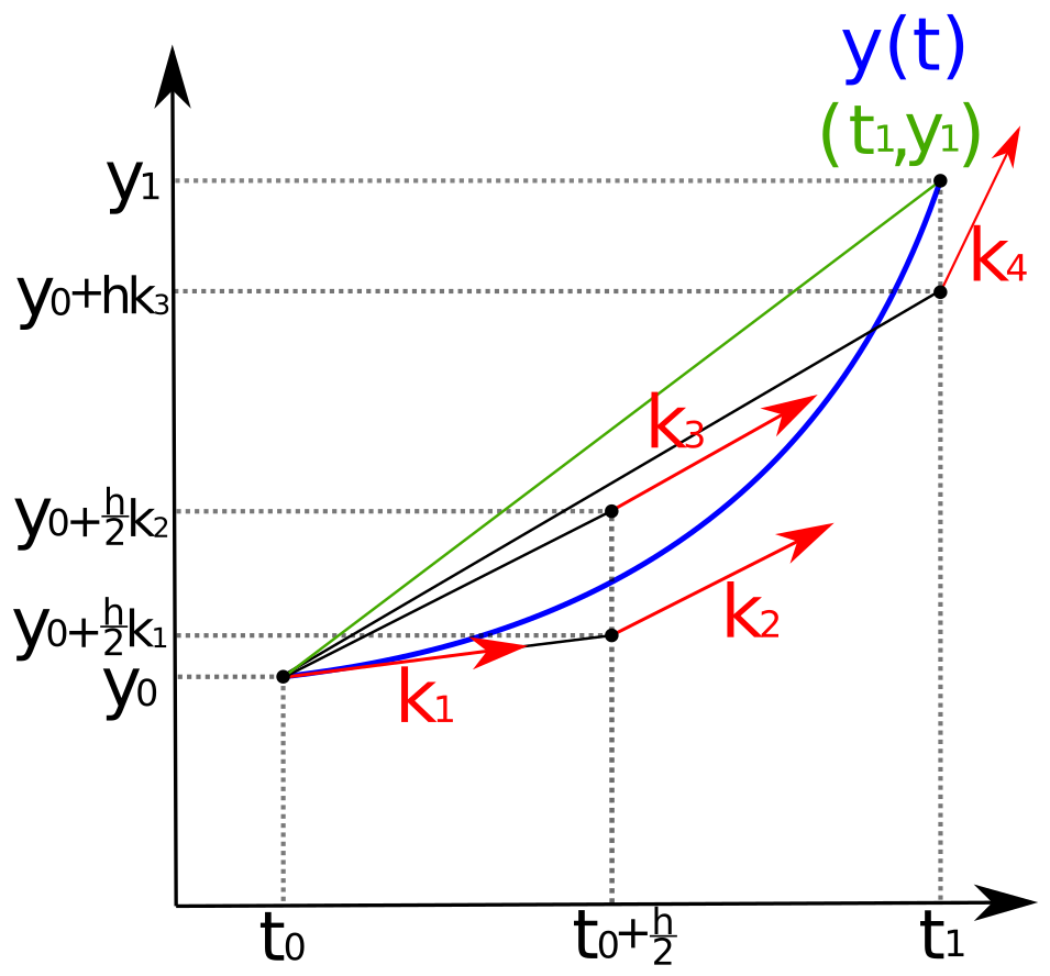
The scheme operates from the initial step \(y_0(t_0)\) to the subsequent step \(y_1(t_1)\) with \(t_1=t_0+h\) and \(y_1=y_0+\phi(t_0,y_0) \cdot h\) by using a weighted increment \(\phi\) calculated from increments \(k_1,..,k_4\). This operation is continued with \(y_1(t_1)\) to estimate \(y_2(t_2)\) an so on.
The increments \(k_1,..,k_4\) are obtained by solving the model equation, as defined in the physical background for the dynamical term \(\frac{dT}{dt}\). The increments differ in their choice of inital conditions (point of evaluation of the model equation). One iterative step always goes through a cycle of evaluating the model equation four times. It starts with the calculation of \(k_1\) at point \(y_0(t_0)\) with:
where \(f(t,y(t))\) is given by the deviation of \(y(t)\), hence \(\frac{dT}{dt} = \frac{1}{C}\cdot(R_{in}+R_{out}+...)\) at \(T_0 (t_0)\).
Now the scheme continues the following procedure:
As final step of one iterative step the weighted increment \(\phi\) is calculated by through:
to estimate \(y_1\) as final step of one iteration step: